factorem belongs to the finRes suite where it facilitates asset pricing research and factor investment backtesting. Install the development version with devtools::install_github("bautheac/factorem").
The package is organised around a workhorse function and a series of wrappers for asset pricing factors popular in the literature. The latter functions get raw financial data retrieved from Bloomberg using the pullit package and return S4 objects that carry data belonging to the corresponding factor including positions and return time series.
factorem
The factorem function is the workhorse function in factorem. From raw financial data and a set of parameter specifications it constructs a complete backtest of the corresponding asset pricing factor and returns the whole time series for the factor positions and returns. For the record the S4 object returned by the function also contains the original raw financial data and the set of parameters supplied as well as the original call to the function. The raw financial data should be supplied in a format similar to that of historical datasets returned by historical data query functions in pullit:
library(pullit); library(lubridate)

tickers_equity <- c("LZB US Equity", "SGA US Equity", "AGCO US Equity", "CLR US Equity",
                    "GHC US Equity", "MAN US Equity", "SITE US Equity", "AJRD US Equity",
                    "COMM US Equity", "GME US Equity", "MEI US Equity", "SMP US Equity")
start <- "2016-01-01"; end <- "2017-12-31"

equity_data_market <- pull_equity_market(source = "Bloomberg", tickers_equity, start, end, verbose = FALSE)

get_data(equity_data_market)
#> ticker field date value
#> 1: AGCO US Equity CUR_MKT_CAP 2016-11-21 4271.793
#> 2: AGCO US Equity CUR_MKT_CAP 2016-11-22 4360.889
#> 3: AGCO US Equity CUR_MKT_CAP 2016-11-23 4507.777
#> 4: AGCO US Equity CUR_MKT_CAP 2016-11-25 4535.067
#> 5: AGCO US Equity CUR_MKT_CAP 2016-11-28 4518.211
#> ---
#> 33466: SMP US Equity PX_VOLUME 2017-12-22 89626.000
#> 33467: SMP US Equity PX_VOLUME 2017-12-26 48762.000
#> 33468: SMP US Equity PX_VOLUME 2017-12-27 119607.000
#> 33469: SMP US Equity PX_VOLUME 2017-12-28 81731.000
#> 33470: SMP US Equity PX_VOLUME 2017-12-29 153615.000From there, construct a bespoke asset pricing factor using the factorem function. I.e., an equity equally weighted momentum factor:
library(factorem)
ranking_period = 1L
factor <- factorem(
name = "momentum", data = pullit::get_data(equity_data_market),
ranking_period = ranking_period, sort_levels = FALSE, weighted = FALSE
)
factor
#> AssetPricingFactor
#> name: momentum factor
#> parameters
#> name: momentum
#> update frequency: month
#> return frequency: day
#> price variable: PX_LAST
#> sort variable: PX_LAST
#> sort levels: FALSE
#> weighted: FALSE
#> ranking period: 1
#> long threshold: 0.5
#> short threshold: 0.5Wrappers
factorem provides wrapper methods for popular asset pricing factors in the literature. At the time of writing the factors covered in the package include, equity market and momentum as well as futures market, momentum, commercial hedging pressure (CHP), open interest and term structure factors. The author welcomes pull requests that would help expanding the current coverage.
Equity
Market
The equity market factor encompasses the entire cross-section of a defined investment opportunity set. It gained popularity in the 1960s for the central role it plays in the Capital Asset Pricing Model (Treynor 1961a, 1961b; Sharpe 1964; Mossin 1966; Lintner 1975) and remains the most popular factor to date in the literature when it comes to explaining the cross-section of equity returns:
equity_market <- market_factor(data = equity_data_market)
equity_market
#> MarketFactor
#> name: equity market factor
#> parameters
#> return frequency: month
#> long: TRUEMomentum
The equity momentum factor is another popular factor in the asset pricing literature. After being first introduced in Carhart (1997) it eventually drew the field leaders’ attention in Fama and French (2012). The equity momentum sorts on prior returns over a defined ranking period:
ranking_period = 1L
equity_momentum <- momentum_factor(data = equity_data_market, ranking_period = ranking_period)
equity_momentum
#> MomentumFactor
#> name: equity momentum factor
#> parameters
#> name: equity momentum
#> update frequency: week
#> return frequency: day
#> price variable: PX_LAST
#> sort variable: PX_LAST
#> sort levels: FALSE
#> weighted: FALSE
#> ranking period: 1
#> long threshold: 0.5
#> short threshold: 0.5Futures
tickers_futures <- c(
'LNA Comdty', 'LPA Comdty', 'LTA Comdty', 'LXA Comdty', 'NGA Comdty', 'O A Comdty',
'PAA Comdty', 'PLA Comdty', 'S A Comdty', 'SBA Comdty', 'SIA Comdty', 'SMA Comdty',
'W A Comdty', 'XBWA Comdty'
)
futures_data_TS <- pull_futures_market(source = "storethat", type = "term structure", tickers_futures,
start, end, file = storethat, verbose = FALSE)
pullit::get_data(futures_data_TS)#> ticker field date value
#> 1: LN1 A:00_0_N Comdty OPEN_INT 2016-01-04 30438
#> 2: LN1 A:00_0_N Comdty OPEN_INT 2016-01-05 30077
#> 3: LN1 A:00_0_N Comdty OPEN_INT 2016-01-06 29828
#> 4: LN1 A:00_0_N Comdty OPEN_INT 2016-01-07 28371
#> 5: LN1 A:00_0_N Comdty OPEN_INT 2016-01-08 28343
#> ---
#> 112006: XBW2 A:00_0_N Comdty PX_VOLUME 2017-12-22 51778
#> 112007: XBW2 A:00_0_N Comdty PX_VOLUME 2017-12-26 50123
#> 112008: XBW2 A:00_0_N Comdty PX_VOLUME 2017-12-27 51936
#> 112009: XBW2 A:00_0_N Comdty PX_VOLUME 2017-12-28 47352
#> 112010: XBW2 A:00_0_N Comdty PX_VOLUME 2017-12-29 44603Market
factorem provides futures equivalent for the factors above including a futures market factor that takes equally weighted positions on the nearby front contract of the commodity futures series provided:
futures_market <- market_factor(data = futures_data_TS)
futures_market
#> MarketFactor
#> name: futures nearby market factor
#> parameters
#> return frequency: month
#> long: TRUEMomentum
The momentum factor is also popular in the futures asset pricing literature in particular in the context of commodity markets (Miffre and Rallis 2007). As does its equity equivalent, it sorts on prior returns:
ranking_period = 1L
futures_momentum <- momentum_factor(data = futures_data_TS, ranking_period = ranking_period)
futures_momentum
#> MomentumFactor
#> name: futures momentum factor
#> parameters
#> name: futures momentum
#> update frequency: week
#> return frequency: day
#> price variable: PX_LAST
#> sort variable: PX_LAST
#> sort levels: FALSE
#> weighted: FALSE
#> ranking period: 1
#> long threshold: 0.5
#> short threshold: 0.5Commercial hedging pressure (CHP)
The futures commercial hedging pressure factor is based on the well-known hedging pressure-based theory (Keynes 1930; Hicks 1939; Houthakker 1957; Cootner 1960) which postulates that futures prices for a given commodity are inversely related to the extent that commercial hedgers are short or long and the mimicking portfolio here aims at capturing the impact of hedging pressure as a systemic factor (Basu and Miffre 2013).
futures_data_CFTC <- pull_futures_CFTC(source = "Bloomberg", tickers_futures, start, end, verbose = FALSE)
ranking_period = 1L
futures_CHP <- CHP_factor(
price_data = futures_data_TS, CHP_data = futures_data_CFTC, ranking_period = ranking_period
)
futures_CHP#> CHPFactor
#> name: CHP factor
#> parameters
#> name: CHP
#> update frequency: month
#> return frequency: day
#> price variable: PX_LAST
#> sort variable: inverse CHP
#> sort levels: TRUE
#> weighted: FALSE
#> ranking period: 1
#> long threshold: 0.5
#> short threshold: 0.5Open interest
The open interest factor relates to futures market liquidity and is also present in the literature where it is described as having explanatory power on the cross-section of commodity futures returns (Hong and Yogo 2012). It comes in two flavours in factorem, nearby and aggregate.
Nearby
The nearby open interest factor is concerned with liquidity at the very front end of the term structure where it sorts on nearby front contract’s open interest:
ranking_period = 1L
futures_OI_nearby <- OI_nearby_factor(data = futures_data_TS, ranking_period = ranking_period)
futures_OI_nearby
#> OIFactor
#> name: nearby OI factor
#> parameters
#> name: nearby OI
#> update frequency: month
#> return frequency: day
#> price variable: PX_LAST
#> sort variable: OPEN_INT
#> sort levels: FALSE
#> weighted: FALSE
#> ranking period: 1
#> long threshold: 0.5
#> short threshold: 0.5Aggregate
In contrast, the aggregate open interest factor is concerned with term structure liquidity as a whole and sorts on open interest summed up over all the contracts of a particular futures series:
futures_data_agg <- pull_futures_market(source = "Bloomberg", type = "aggregate", tickers_futures,
start, end, verbose = FALSE)
ranking_period = 1L
futures_OI_aggregate <- OI_aggregate_factor(price_data = futures_data_market,
aggregate_data = futures_data_agg,
ranking_period = ranking_period)#> OIFactor
#> name: aggregate OI factor
#> parameters
#> name: aggregate OI
#> update frequency: month
#> return frequency: day
#> price variable: PX_LAST
#> sort variable: FUT_AGGTE_OPEN_INT
#> sort levels: FALSE
#> weighted: FALSE
#> ranking period: 1
#> long threshold: 0.5
#> short threshold: 0.5Term structure
The futures term structure factor (Szymanowska et al. 2014; Fuertes, Miffre, and Fernandez-Perez 2015) is concerned with the shape (steepness) of the futures term structure and sorts on roll yield:
ranking_period = 1L
futures_TS <- TS_factor(data = futures_data_TS, ranking_period = ranking_period)
futures_TS
#> TSFactor
#> name: futures term structure factor
#> parameters
#> name: futures term structure
#> update frequency: month
#> return frequency: day
#> price variable: PX_LAST
#> sort variable: carry
#> sort levels: TRUE
#> weighted: FALSE
#> ranking period: 1
#> long threshold: 0.5
#> short threshold: 0.5Accessors
Accessor methods allow access to the content of the factor objects returned by the functions described above: ### Name
get_name(factor)
#> [1] "momentum"Positions
get_positions(factor)
#> date name position
#> 1: 2016-12-30 LZB US Equity long
#> 2: 2016-12-30 MEI US Equity long
#> 3: 2016-12-30 SMP US Equity long
#> 4: 2016-12-30 SGA US Equity long
#> 5: 2016-12-30 GHC US Equity long
#> ---
#> 152: 2017-12-29 SGA US Equity short
#> 153: 2017-12-29 LZB US Equity short
#> 154: 2017-12-29 GME US Equity short
#> 155: 2017-12-29 GHC US Equity short
#> 156: 2017-12-29 MAN US Equity shortReturns
get_returns(factor)
#> date long short factor
#> 1: 2017-01-03 0.0135047148 -0.0109830009 0.0012608570
#> 2: 2017-01-04 0.0143650103 -0.0218710531 -0.0037530214
#> 3: 2017-01-05 -0.0324683966 0.0101188617 -0.0111747674
#> 4: 2017-01-06 0.0009696990 0.0112154077 0.0060925534
#> 5: 2017-01-09 -0.0068085180 0.0063287768 -0.0002398706
#> ---
#> 247: 2017-12-22 -0.0007898250 0.0101846620 0.0046974185
#> 248: 2017-12-26 0.0093618073 0.0063778750 0.0078698411
#> 249: 2017-12-27 -0.0001223505 -0.0012346003 -0.0006784754
#> 250: 2017-12-28 -0.0001494908 0.0008308516 0.0003406804
#> 251: 2017-12-29 -0.0059587926 0.0079990948 0.0010201511Data initially supplied
factorem::get_data(factor)
#>                ticker       field       date      value
#>     1: AGCO US Equity CUR_MKT_CAP 2016-11-21   4271.793
#>     2: AGCO US Equity CUR_MKT_CAP 2016-11-22   4360.889
#>     3: AGCO US Equity CUR_MKT_CAP 2016-11-23   4507.777
#>     4: AGCO US Equity CUR_MKT_CAP 2016-11-25   4535.067
#>     5: AGCO US Equity CUR_MKT_CAP 2016-11-28   4518.211
#>    ---
#> 33466:  SMP US Equity   PX_VOLUME 2017-12-22  89626.000
#> 33467:  SMP US Equity   PX_VOLUME 2017-12-26  48762.000
#> 33468:  SMP US Equity   PX_VOLUME 2017-12-27 119607.000
#> 33469:  SMP US Equity   PX_VOLUME 2017-12-28  81731.000
#> 33470: SMP US Equity PX_VOLUME 2017-12-29 153615.000Parameters
get_parameters(factor)
#>            parameter    value
#>  1:             name momentum
#>  2: update frequency    month
#>  3: return frequency      day
#>  4:   price variable  PX_LAST
#>  5:    sort variable  PX_LAST
#>  6:      sort levels    FALSE
#>  7:         weighted    FALSE
#>  8:   ranking_period        1
#>  9:   long_threshold      0.5
#> 10:  short_threshold      0.5
Function call
factorem::get_call(factor)
#> factorem(name = "momentum", data = pullit::get_data(equity_data_market),
#>     sort_levels = FALSE, weighted = FALSE, ranking_period = ranking_period)
Summary
A summary method returns a performance summary of the corresponding factor:
summary(factor)
#>   year      Jan     Feb     Mar      Apr      May      Jun      Jul      Aug
#> 1 2017 -0.01362 0.01101 0.03168 -0.00643 -0.00806 -0.00909 -0.00299 -0.01587
#>        Sep     Oct     Nov     Dec   total
#> 1 -0.00367 0.00101 0.04334 0.03185 0.05851
plotit
The plotit package, also part of the finRes suite, provides plot methods for the factor objects returned by the functions above:
performance overview
The plot function dispatched on a factor object from factorem with the parameter type set to “performance” displays an overview of the performance of the corresponding factor in the form of equity curves. The equity curve for the factor is plotted along with, for long-short factors only, that of the long and short legs of the factor independently:
positions overview
Similarly, with the type parameter set to “positions”, the plot function shows the proportion of time each asset leaves in the factor with a breakdown by leg for long-short factors:
plot(factor, type = "positions")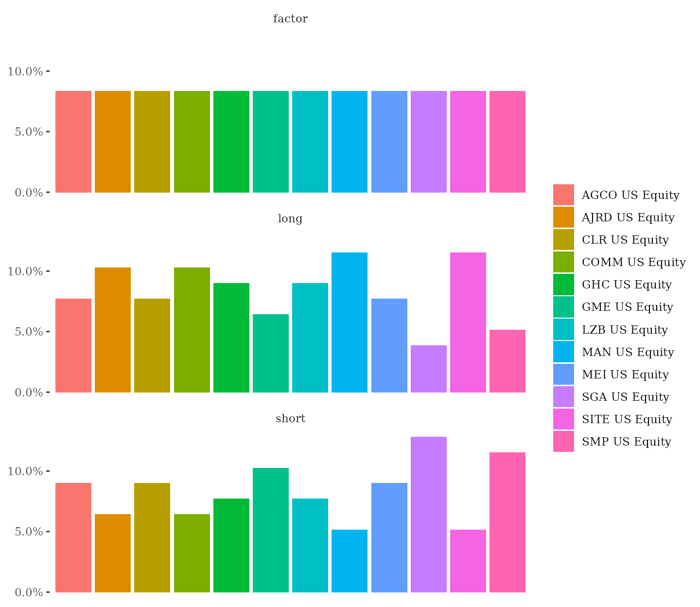
References
Basu, Devraj, and Joëlle Miffre. 2013. “Capturing the Risk Premium of Commodity Futures: The Role of Hedging Pressure.” Journal of Banking & Finance 37 (7): 2652–64. https://doi.org/10.1016/j.jbankfin.2013.02.031.
Carhart, Mark M. 1997. “On Persistence in Mutual Fund Performance.” The Journal of Finance 52 (1): 57–82.
Cootner, Paul H. 1960. “Returns to Speculators: Telser Versus Keynes.” Journal of Political Economy 68 (4): 396–404. https://doi.org/10.1086/258347.
Fama, Eugene F., and Kenneth R. French. 2012. “Size, Value, and Momentum in International Stock Returns.” Journal of Financial Economics 105 (3): 457–72.
Fuertes, Ana-Maria, Joëlle Miffre, and Adrian Fernandez-Perez. 2015. “Commodity Strategies Based on Momentum, Term Structure, and Idiosyncratic Volatility.” Journal of Futures Markets 35 (3): 274–97. https://doi.org/10.1002/fut.21656.
Hicks, John Richard. 1939. Value and Capital. 1st ed. Oxford University Press, Cambridge.
Hong, Harrison, and Motohiro Yogo. 2012. “What Does Futures Market Interest Tell Us About the Macroeconomy and Asset Prices?” Journal of Financial Economics 105 (3): 473–90. https://doi.org/10.1016/j.jfineco.2012.04.005.
Houthakker, Hendrik. 1957. “Restatement of the Theory of Normal Backwardation.” Cowles Foundation Discussion Papers 44. Cowles Foundation for Research in Economics, Yale University. https://EconPapers.repec.org/RePEc:cwl:cwldpp:44.
Keynes, John Maynard. 1930. Treatise on Money. Macmillan, London.
Lintner, John. 1975. “The Valuation of Risk Assets and the Selection of Risky Investments in Stock Portfolios and Capital Budgets.” In Stochastic Optimization Models in Finance, 131–55. Elsevier.
Miffre, Joëlle, and Georgios Rallis. 2007. “Momentum Strategies in Commodity Futures Markets.” Journal of Banking & Finance 31 (6): 1863–86.
Mossin, Jan. 1966. “Equilibrium in a Capital Asset Market.” Econometrica 34 (4): 768–83. https://doi.org/10.2307/1910098.
Sharpe, William F. 1964. “Capital Asset Prices: A Theory of Market Equilibrium Under Conditions of Risk.” The Journal of Finance 19 (3): 425–42.
Szymanowska, Marta, Frans De Roon, Theo Nijman, and Rob Van Den Goorbergh. 2014. “An Anatomy of Commodity Futures Risk Premia.” The Journal of Finance 69 (1): 453–82. https://doi.org/10.1111/jofi.12096.
Treynor, Jack L. 1961a. “Market Value, Time, and Risk.”
———. 1961b. Toward a Theory of Market Value of Risky Assets.